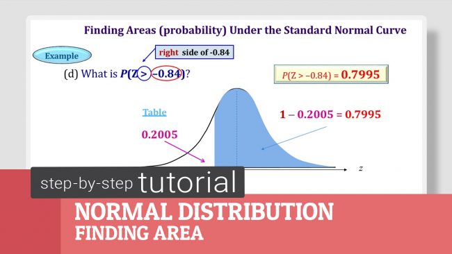
The Normal Distribution Finding Area
Tutorial Video

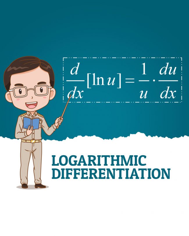
In this video, you’ll learn about logarithmic differentiation, a powerful technique in calculus used to differentiate complex functions, particularly those involving products, quotients, or exponents.
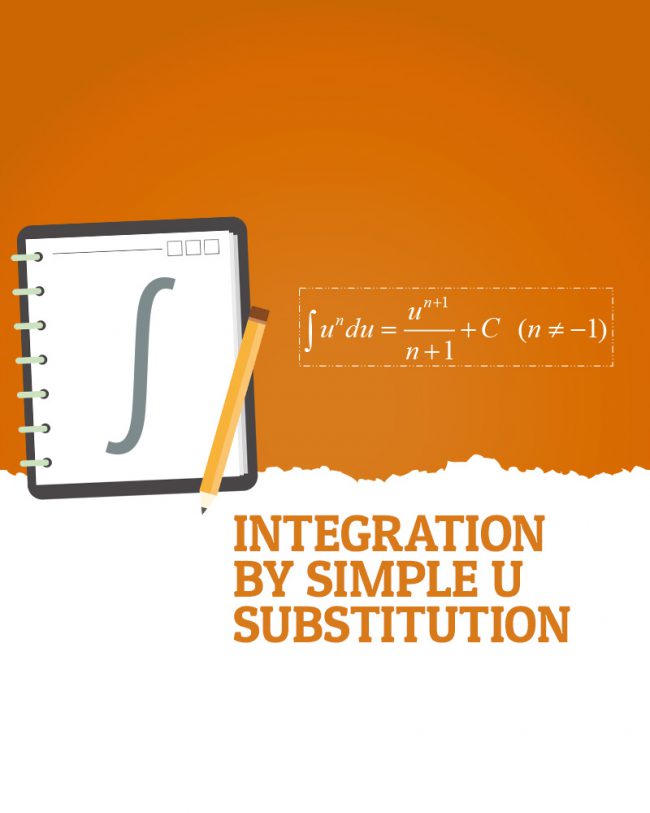
[tlg_steps style=”steps-style-2″][tlg_steps_content step_link=”url:http%3A%2F%2F127.0.0.1%2Fmkmath%2Fcalculus%2F” title=”Calculus” icon=”ti-arrow-circle-right” subtitle=”Topics”][tlg_steps_content title=”Integration” icon=”ti-arrow-circle-right” subtitle=”Topics”][/tlg_steps] This method allows us to differentiate very complicated fractional functions or functions raised to the power of another function easily. More in this Section [tlg_blog layout=”carouseldetail” pppage=”-1″ pagination=”yes” overlay=”no-overlay” filter=”452″]
[tlg_steps style=”steps-style-2″][tlg_steps_content step_link=”url:http%3A%2F%2F127.0.0.1%2Fmkmath%2Fcalculus%2F” title=”Calculus” icon=”ti-arrow-circle-right” subtitle=”Topics”][tlg_steps_content step_link=”url:http%3A%2F%2F127.0.0.1%2Fmkmath%2Fcalculus%2Fintro%2F|title:Introductory%20Calculus” title=”General” icon=”ti-arrow-circle-right” subtitle=”Topics”][/tlg_steps] Here are tips for graphing. First, you need to find x-intercepts and y-intercept, if possible. For x-intercepts, setting y=0 to find x-values and similarly, setting x=0 to find y-intercept. Then, investigate if there are any asymptotes for fractional functions. For the horizontal asymptotes, we need…
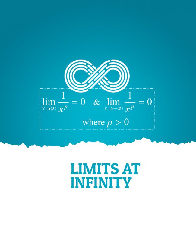
[tlg_steps style=”steps-style-2″][tlg_steps_content step_link=”url:http%3A%2F%2F127.0.0.1%2Fmkmath%2Fcalculus%2F” title=”Calculus” icon=”ti-arrow-circle-right” subtitle=”Topics”][tlg_steps_content step_link=”url:http%3A%2F%2F127.0.0.1%2Fmkmath%2Fcalculus%2Fintro%2F|title:Introductory%20Calculus” title=”Introductory” icon=”ti-arrow-circle-right” subtitle=”Topics”][/tlg_steps] To evaluate the limit as x approaches infinity, take the largest exponent term each from the numerator and denominator, simplify the fraction, and then apply the limit rules as shown. More in this Section [tlg_blog layout=”carouseldetail” pppage=”-1″ pagination=”yes” overlay=”no-overlay” filter=”455″]
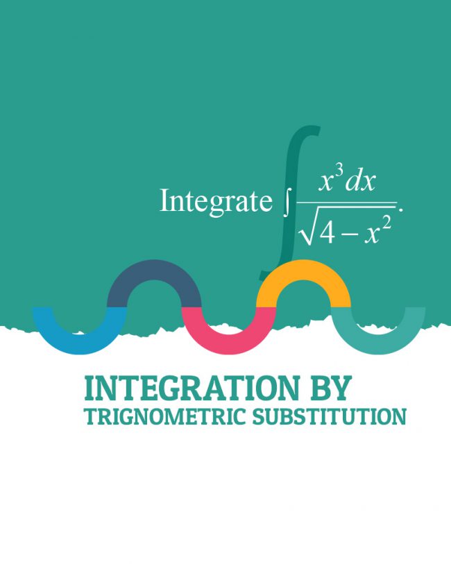
[tlg_steps style=”steps-style-2″][tlg_steps_content step_link=”url:http%3A%2F%2F127.0.0.1%2Fmkmath%2Fcalculus%2F” title=”Calculus” icon=”ti-arrow-circle-right” subtitle=”Topics”][tlg_steps_content step_link=”url:http%3A%2F%2F127.0.0.1%2Fmkmath%2Fcalculus%2Fintegration%2F|title:Introductory%20Calculus” title=”Integration” icon=”ti-arrow-circle-right” subtitle=”Topics”][/tlg_steps] This method allows us to change algebraic functions into trigonometric functions, integrate them in trigonometric forms, and return to the original algebraic functions as solutions. More in this Section [tlg_blog layout=”carouseldetail” pppage=”-1″ pagination=”yes” overlay=”no-overlay” filter=”452″]
[tlg_steps style=”steps-style-2″][tlg_steps_content step_link=”url:http%3A%2F%2F127.0.0.1%2Fmkmath%2Fcalculus%2F” title=”Calculus” icon=”ti-arrow-circle-right” subtitle=”Topics”][tlg_steps_content step_link=”url:http%3A%2F%2F127.0.0.1%2Fmkmath%2Fcalculus%2Fintro%2F|title:Introductory%20Calculus” title=”General” icon=”ti-arrow-circle-right” subtitle=”Topics”][/tlg_steps] Before starting the example, you need to know the following steps to solve DE by Laplace transforms. Step 1. Take the Laplace transforms of both sides of the equation. Step 2. Solve for the Laplace of Y. Step 3. Manipulate the Laplace transform, F(s) until…